从大三到现在一直在学习机器学习相关的理论,可是隐约间觉得自己对于机器学习算法的理解还只是停留在理论层面,理解还是很浅薄的,并不深刻。此外,最近听到了一些关于机器学习理论与实践关系的说法,觉得挺有道理的,摘录如下:

• 只有真正将机器学习算法应用到某个具体问题上的时候,你的学习才刚刚开始。
• 机器学习的过程实际上是一个学习理论、实践、学习理论、实践...的过程,只有经过这样一轮又一轮的过滤,你才能慢慢的开始理解机器学习算法。从哲学上来说,其实这就是一个理论联系实际的过程。
• Talk is cheap,show me your code.
• When I cannot create,I do not understand.

总而言之,言而总之,婶婶地觉得我该实践实践了,真正针对实际问题,动手去实现一些机器学习算法,并检验它们的实际效果。

作为机器学习实战系列的第一篇,本博文选取的问题来自Kaggle,我选取了Digit Recognizer这个问题,于是牛刀霍霍,开始解剖这个问题。

根据该问主页上的提示,我打算实现Random Forest以及Convolutional Network来检验这两个问题针对手写数字识别这个问题的实际应用效果,以下就记录一下整个过程吧。

随机森林

随机森林算法是在决策树算法的基础上提出,关于决策树算法的相关知识可参考我之前写的一篇机器学习系列(I):决策树算法,它的核心思想是随机选取训练样本以及随机选取特征,从而针对这些训练样本以及随机选取的特征根据决策树算法构建多棵决策树,最后综合多棵决策树的结果得出须预测样本的分类。由于之前实现过决策树算法,于是这里我就不想实现这个算法了,具体采用scikit工具包中提供的随机森林分类器进行训练。

具体实现时,由于Kaggle提供的测试集是以csv格式提供的,在一大通搜索之后,我最后采用了pandas库处理文件输入及输出问题,根据其官网上的说明:

Pandas is an open source, BSD-licensed library providing high-performance, easy-to-use data structures and data analysis tools for the Python programming language.

可见pandas是针对python开发的一个高性能且易用的数据结构以及数据分析工具库。在处理Kaggle数据的时候用了一下,个人感觉还是挺好用的。

另外需要说明的一点是,面对MNIST数据集的时候,最先想到的一个问题是如何提取特征以用于手写数字识别的问题中,大概查了一下,一种比较简单的方法是将整个图像分成很多不重叠的2*2的小区域,然后统计每个小区域中不为0的像素值的总数(另,可针对不同的区域设置不同的权重)。在查找的过程中也发现了很多其他方法,有兴趣的朋友可以自行Google之。因为Kaggle提供的训练集每张图片都是一个长度为784的长向量,个人觉得计算2*2小区域包含不为0像素的总数不是很方便(现在看来还是挺简单的昂),所以直接一股脑地把整个784位的向量作为特征扔给随机森林分类器了。(唉,现在觉得自己太不负责任了,怎么能够这样呢?).以下给出采用随机森林进行训练的源代码。

#-*- coding:utf-8 -*-
import numpy as np
import pandas as pd
from sklearn.ensemble import RandomForestClassifier

'''
A simple random forest program for minist digit recognition
@author:qingyuanxingsi
@date:2014/05/11
'''

csvPath = '/home/qingyuanxingsi/data/digit_recognizer/train.csv'
testPath = '/home/qingyuanxingsi/data/digit_recognizer/test.csv'
destPath = '/home/qingyuanxingsi/data/digit_recognizer/result.csv'
n_samples = 42000

#Loading the csv data
digitArray = pd.read_csv(csvPath).as_matrix()

#Split the data into two parts:data and tag
dataArray = digitArray[:,1:]
tagArray = digitArray[:,0:1].reshape(n_samples,)

#Feed the data and tag into the random forest classifier of the scikit toolkit

randomForestClassifier = RandomForestClassifier(n_estimators = 10)
randomForestClassifier.fit(dataArray,tagArray)

#Read the test dat in
testDat = pd.read_csv(testPath).as_matrix()

tags = []
for i in range(testDat.shape[0]):
    tags.append(randomForestClassifier.predict(testDat[i]))

pd.Series(tags).to_csv(destPath,index=True)

得到分析结果并提交到Kaggle之后,最后的准确率没我想象的那么惨不忍睹,Kaggle选取部分测试集进行测试之后给的SCORE是94%左右,效果也不是灰常灰常差啦。

当然,这个准确率个人实在不是很满意,所以打算拿Convolutional Neural Network试试。

卷积神经网络

概述

卷积神经网络是一种特殊的深层的神经网络模型，它的特殊性体现在两个方面，一方面它的神经元间的连接是非全连接的，另一方面同一层中某些神经元之间的连接的权重是共享的（即相同的）。它的非全连接和权值共享的网络结构使之更类似于生物神经网络，降低了网络模型的复杂度（对于很难学习的深层结构来说，这是非常重要的），减少了权值的数量。

卷积网络最初是受视觉神经机制的启发而设计的，是为识别二维形状而设计的一个多层感知器，这种网络结构对平移、比例缩放、倾斜或者其他形式的变形具有高度不变性。1962年Hubel和Wiesel通过对猫视觉皮层细胞的研究，提出了感受野(receptive field)的概念，1984年日本学者Fukushima基于感受野概念提出的神经认知机(neocognitron)模型，它可以看作是卷积神经网络的第一个实现网络，也是感受野概念在人工神经网络领域的首次应用。

神经认知机将一个视觉模式分解成许多子模式(特征)，然后进入分层递阶式相连的特征平面进行处理，它试图将视觉系统模型化，使其能够在即使物体有位移或轻微变形的时候，也能完成识别。神经认知机能够利用位移恒定能力从激励模式中学习，并且可识别这些模式的变化形。在其后的应用研究中，Fukushima将神经认知机主要用于手写数字的识别。随后，国内外的研究人员提出多种卷积神经网络形式，在邮政编码识别（Y. LeCun etc）、车牌识别和人脸识别等方面得到了广泛的应用。

CNN的结构

卷积网络是为识别二维形状而特殊设计的一个多层感知器，这种网络结构对平移、比例缩放、倾斜或者共他形式的变形具有高度不变性。 这些良好的性能是网络在有监督方式下学会的，网络的结构主要有稀疏连接和权值共享两个特点，包括如下形式的约束：

• 特征提取。每一个神经元从上一层的局部接受域得到突触输人，因而迫使它提取局部特征。一旦一个特征被提取出来，只要它相对于其他特征的位置被近似地保留下来，它的精确位置就变得没有那么重要了。
• 特征映射。网络的每一个计算层都是由多个特征映射组成的，每个特征映射都是平面形式的。平面中单独的神经元在约束下共享相同的突触权值集，这种结构形式具有如下的有益效果：a.平移不变性。b.自由参数数量的缩减(通过权值共享实现)。
• 子抽样。每个卷积层跟着一个实现局部平均和子抽样的计算层，由此特征映射的分辨率降低。这种操作具有使特征映射的输出对平移和其他形式的变形的敏感度下降的作用。

稀疏连接(Sparse Connectivity)

卷积网络通过在相邻两层之间强制使用局部连接模式来利用图像的空间局部特性，在第$m$层的隐层单元只与第$m-1$层的输入单元的局部区域有连接，第$m-1$层的这些局部区域被称为空间连续的接受域。我们可以将这种结构描述如下：设第$m-1$层为视网膜输入层，第$m$层的接受域的宽度为3，也就是说该层的每个单元与且仅与输入层的3个相邻的神经元相连，第$m$层与第$m+1$层具有类似的链接规则，如下图所示。

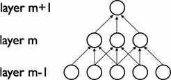
可以看到$m+1$层的神经元相对于第$m$层的接受域的宽度也为3，但相对于输入层的接受域为5，这种结构将学习到的过滤器（对应于输入信号中被最大激活的单元)限制在局部空间模式（因为每个单元对它接受域外的variation不做反应）。从上图也可以看出，多个这样的层堆叠起来后，会使得过滤器（不再是线性的）逐渐成为全局的（也就是覆盖到了更大的视觉区域）。例如上图中第$m+1$层的神经元可以对宽度为5的输入进行一个非线性的特征编码。

权值共享(Shared Weights)

在卷积网络中，每个稀疏过滤器$h_i$通过共享权值都会覆盖整个可视域，这些共享权值的单元构成一个特征映射，如下图所示:

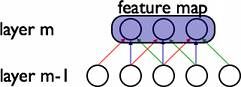
在图中，有3个隐层单元，他们属于同一个特征映射。同种颜色的链接的权值是相同的，我们仍然可以使用梯度下降的方法来学习这些权值，只需要对原始算法做一些小的改动，这里共享权值的梯度是所有共享参数的梯度的总和。我们不禁会问为什么要权重共享呢？一方面，重复单元能够对特征进行识别，而不考虑它在可视域中的位置。另一方面，权值共享使得我们能更有效的进行特征抽取，因为它极大的减少了需要学习的自由变量的个数。通过控制模型的规模，卷积网络对视觉问题可以具有很好的泛化能力。

The Full Model

卷积神经网络是一个多层的神经网络，每层由多个二维平面组成，而每个平面由多个独立神经元组成。网络中包含一些简单元和复杂元，分别记为S-元和C-元。S-元聚合在一起组成S-面，S-面聚合在一起组成S-层，用Us表示。C-元、C-面和C-层($U_s$)之间存在类似的关系。网络的任一中间级由S-层与C-层串接而成，而输入级只含一层，它直接接受二维视觉模式，样本特征提取步骤已嵌入到卷积神经网络模型的互联结构中。

一般地，$U_s$为特征提取层，每个神经元的输入与前一层的局部感受野相连，并提取该局部的特征，一旦该局部特征被提取后，它与其他特征间的位置关系 也随之确定下来；$U_c$是特征映射层，网络的每个计算层由多个特征映射组成，每个特征映射为一个平面，平面上所有神经元的权值相等。特征映射结构采用影响函数核小的sigmoid函数作为卷积网络的激活函数，使得特征映射具有位移不变性(这一句表示没看懂，那位如果看懂了，请给我讲解一下)。此外，由于一个映射面上的神经元共享权值，因而减少了网络自由参数的个数，降低了网络参数选择的复杂度。卷积神经网络中的每一个特征提取层(S-层)都紧跟着一个用来求局部平均与二次提取的计算层(C-层)，这种特有的两次特征提取结构使网络在识别时对输入样本有较高的畸变容忍能力。

下图是一个卷积网络的实例:

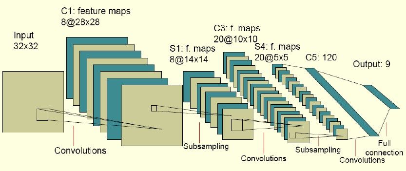
图中的卷积网络工作流程如下，输入层由32×32个感知节点组成，接收原始图像。然后，计算流程在卷积和子抽样之间交替进行，如下所 述：第一隐藏层进行卷积，它由8个特征映射组成，每个特征映射由28×28个神经元组成，每个神经元指定一个5×5的接受域；第二隐藏层实现子 抽样和局部平均，它同样由8个特征映射组成，但其每个特征映射由14×14个神经元组成。每个神经元具有一个 2×2 的接受域，一个可训练系数，一个可训练偏置和一个sigmoid激活函数。可训练系数和偏置控制神经元的操作点。第三隐藏层进行第二次卷积，它由20个特征映射组成每个特征映射由10×10个神经元组成。该隐藏层中的每个神经元可能具有和下一个隐藏层几个特征映射相连的突触连接，它以与第一个卷积层相似的方式操作。第四个隐藏层进行第二次子抽样和局部平均汁算。它由20个特征映射组成，但每个特征映射由5×5个神经元组成，它以与第一次抽样相似的方式操作。第五个隐藏层实现卷积的最后阶段，它由 120 个神经元组成，每个神经元指定一个5×5的接受域。最后是个全连接层，得到输出向量。相继的计算层在卷积和抽样之间的连续交替，我们得到一个“双尖塔”的效果，也就是在每个卷积或抽样层，随着空间分辨率下降，与相应的前一层相比特征映射的数量增加。卷积之后进行子抽样的思想是受到动物视觉系统中的“简单的”细胞后面跟着“复杂的”细胞的想法的启发而产生的。图中所示的多层感知器包含近似100000个突触连接，但只有大约2600个自由参数。自由参数在数量上显著地减少是通过权值共享获得 的，学习机器的能力（以VC维的形式度量）因而下降，这又提高它的泛化能力。而且它对自由参数的调整通过反向传播学习的随机形式来实 现。另一个显著的特点是使用权值共享使得以并行形式实现卷积网络变得可能。这是卷积网络对全连接的多层感知器而言的另一个优点。

以上我们简要介绍了一下卷积神经网络的基本概念和基本架构,如何对每个部分进行简单的代码实现可参考Convolutional Neural Networks (LeNet),里面对如何对卷积以及Pooling进行代码实现做了粗略的介绍。实际上,我构建的用于识别手写数字的程序也是在以上代码的基础上理解之后稍加修改后形成的。以下给出具体代码(以下代码中mlp以及logistic_sgd模块可从文字上给出的链接处下载):

import cPickle
import gzip
import os
import sys
import time

import numpy

import theano
import theano.tensor as T
from theano.tensor.signal import downsample
from theano.tensor.nnet import conv

from logistic_sgd import LogisticRegression, load_data
from mlp import HiddenLayer
import pandas as pd


class LeNetConvPoolLayer(object):
    """Pool Layer of a convolutional network """

    def __init__(self, rng, input, filter_shape, image_shape, poolsize=(2, 2)):
        """
        Allocate a LeNetConvPoolLayer with shared variable internal parameters.

        :type rng: numpy.random.RandomState
        :param rng: a random number generator used to initialize weights

        :type input: theano.tensor.dtensor4
        :param input: symbolic image tensor, of shape image_shape

        :type filter_shape: tuple or list of length 4
        :param filter_shape: (number of filters, num input feature maps,
                              filter height,filter width)

        :type image_shape: tuple or list of length 4
        :param image_shape: (batch size, num input feature maps,
                             image height, image width)

        :type poolsize: tuple or list of length 2
        :param poolsize: the downsampling (pooling) factor (#rows,#cols)
        """

        assert image_shape[1] == filter_shape[1]
        self.input = input

        # there are "num input feature maps * filter height * filter width"
        # inputs to each hidden unit
        fan_in = numpy.prod(filter_shape[1:])
        # each unit in the lower layer receives a gradient from:
        # "num output feature maps * filter height * filter width" /
        #   pooling size
        fan_out = (filter_shape[0] * numpy.prod(filter_shape[2:]) /
                   numpy.prod(poolsize))
        # initialize weights with random weights
        W_bound = numpy.sqrt(6. / (fan_in + fan_out))
        self.W = theano.shared(numpy.asarray(
            rng.uniform(low=-W_bound, high=W_bound, size=filter_shape),
            dtype=theano.config.floatX),
                               borrow=True)

        # the bias is a 1D tensor -- one bias per output feature map
        b_values = numpy.zeros((filter_shape[0],), dtype=theano.config.floatX)
        self.b = theano.shared(value=b_values, borrow=True)

        # convolve input feature maps with filters
        conv_out = conv.conv2d(input=input, filters=self.W,
                filter_shape=filter_shape, image_shape=image_shape)

        # downsample each feature map individually, using maxpooling
        pooled_out = downsample.max_pool_2d(input=conv_out,
                                            ds=poolsize, ignore_border=True)

        # add the bias term. Since the bias is a vector (1D array), we first
        # reshape it to a tensor of shape (1,n_filters,1,1). Each bias will
        # thus be broadcasted across mini-batches and feature map
        # width & height
        self.output = T.tanh(pooled_out + self.b.dimshuffle('x', 0, 'x', 'x'))

        # store parameters of this layer
        self.params = [self.W, self.b]


def evaluate_lenet5(learning_rate=0.1, n_epochs=200,
                    dataset='/home/qingyuanxingsi/data/digit_recognizer/mnist.pkl.gz',
                    nkerns=[20, 50], batch_size=500):
    """ Demonstrates lenet on MNIST dataset

    :type learning_rate: float
    :param learning_rate: learning rate used (factor for the stochastic
                          gradient)

    :type n_epochs: int
    :param n_epochs: maximal number of epochs to run the optimizer

    :type dataset: string
    :param dataset: path to the dataset used for training /testing (MNIST here)

    :type nkerns: list of ints
    :param nkerns: number of kernels on each layer
    """

    rng = numpy.random.RandomState(23455)

    datasets = load_data(dataset)

    train_set_x, train_set_y = datasets[0]
    valid_set_x, valid_set_y = datasets[1]
    test_set_x, test_set_y = datasets[2]

    #import my own dataset
    predict_set = pd.read_csv('/home/qingyuanxingsi/data/digit_recognizer/test.csv').as_matrix()
    predict_set = predict_set/256.0
    predict_set_x = theano.shared(numpy.asarray(predict_set,
                                               dtype=theano.config.floatX),
                                 borrow=True)
    predict_set_tag = numpy.zeros([predict_set.shape[0],])

    # compute number of minibatches for training, validation and testing
    n_train_batches = train_set_x.get_value(borrow=True).shape[0]
    n_valid_batches = valid_set_x.get_value(borrow=True).shape[0]
    n_test_batches = test_set_x.get_value(borrow=True).shape[0]
    n_predict_batches = predict_set_x.get_value(borrow=True).shape[0]
    n_train_batches /= batch_size
    n_valid_batches /= batch_size
    n_test_batches /= batch_size
    n_predict_batches /= batch_size

    # allocate symbolic variables for the data
    index = T.lscalar()  # index to a [mini]batch
    x = T.matrix('x')   # the data is presented as rasterized images
    y = T.ivector('y')  # the labels are presented as 1D vector of
                        # [int] labels

    ishape = (28, 28)  # this is the size of MNIST images

    ######################
    # BUILD ACTUAL MODEL #
    ######################
    print '... building the model'

    # Reshape matrix of rasterized images of shape (batch_size,28*28)
    # to a 4D tensor, compatible with our LeNetConvPoolLayer
    layer0_input = x.reshape((batch_size, 1, 28, 28))

    # Construct the first convolutional pooling layer:
    # filtering reduces the image size to (28-5+1,28-5+1)=(24,24)
    # maxpooling reduces this further to (24/2,24/2) = (12,12)
    # 4D output tensor is thus of shape (batch_size,nkerns[0],12,12)
    layer0 = LeNetConvPoolLayer(rng, input=layer0_input,
            image_shape=(batch_size, 1, 28, 28),
            filter_shape=(nkerns[0], 1, 5, 5), poolsize=(2, 2))

    # Construct the second convolutional pooling layer
    # filtering reduces the image size to (12-5+1,12-5+1)=(8,8)
    # maxpooling reduces this further to (8/2,8/2) = (4,4)
    # 4D output tensor is thus of shape (nkerns[0],nkerns[1],4,4)
    layer1 = LeNetConvPoolLayer(rng, input=layer0.output,
            image_shape=(batch_size, nkerns[0], 12, 12),
            filter_shape=(nkerns[1], nkerns[0], 5, 5), poolsize=(2, 2))

    # the HiddenLayer being fully-connected, it operates on 2D matrices of
    # shape (batch_size,num_pixels) (i.e matrix of rasterized images).
    # This will generate a matrix of shape (20,32*4*4) = (20,512)
    layer2_input = layer1.output.flatten(2)

    # construct a fully-connected sigmoidal layer
    layer2 = HiddenLayer(rng, input=layer2_input, n_in=nkerns[1] * 4 * 4,
                         n_out=500, activation=T.tanh)

    # classify the values of the fully-connected sigmoidal layer
    layer3 = LogisticRegression(input=layer2.output, n_in=500, n_out=10)

    # the cost we minimize during training is the NLL of the model
    cost = layer3.negative_log_likelihood(y)

    # create a function to compute the mistakes that are made by the model
    test_model = theano.function([index], layer3.errors(y),
             givens={
                x: test_set_x[index * batch_size: (index + 1) * batch_size],
                y: test_set_y[index * batch_size: (index + 1) * batch_size]})

    validate_model = theano.function([index], layer3.errors(y),
            givens={
                x: valid_set_x[index * batch_size: (index + 1) * batch_size],
                y: valid_set_y[index * batch_size: (index + 1) * batch_size]})

    # create a list of all model parameters to be fit by gradient descent
    params = layer3.params + layer2.params + layer1.params + layer0.params

    # create a list of gradients for all model parameters
    grads = T.grad(cost, params)

    # train_model is a function that updates the model parameters by
    # SGD Since this model has many parameters, it would be tedious to
    # manually create an update rule for each model parameter. We thus
    # create the updates list by automatically looping over all
    # (params[i],grads[i]) pairs.
    updates = []
    for param_i, grad_i in zip(params, grads):
        updates.append((param_i, param_i - learning_rate * grad_i))

    train_model = theano.function([index], cost, updates=updates,
          givens={
            x: train_set_x[index * batch_size: (index + 1) * batch_size],
            y: train_set_y[index * batch_size: (index + 1) * batch_size]})

    ###############
    # TRAIN MODEL #
    ###############
    print '... training'
    # early-stopping parameters
    patience = 10000  # look as this many examples regardless
    patience_increase = 2  # wait this much longer when a new best is
                           # found
    improvement_threshold = 0.995  # a relative improvement of this much is
                                   # considered significant
    validation_frequency = min(n_train_batches, patience / 2)
                                  # go through this many
                                  # minibatche before checking the network
                                  # on the validation set; in this case we
                                  # check every epoch

    best_params = None
    best_validation_loss = numpy.inf
    best_iter = 0
    test_score = 0.
    start_time = time.clock()

    epoch = 0
    done_looping = False

    while (epoch < n_epochs) and (not done_looping):
        epoch = epoch + 1
        for minibatch_index in xrange(n_train_batches):

            iter = (epoch - 1) * n_train_batches + minibatch_index

            if iter % 100 == 0:
                print 'training @ iter = ', iter
            cost_ij = train_model(minibatch_index)

            if (iter + 1) % validation_frequency == 0:

                # compute zero-one loss on validation set
                validation_losses = [validate_model(i) for i
                                     in xrange(n_valid_batches)]
                this_validation_loss = numpy.mean(validation_losses)
                print('epoch %i, minibatch %i/%i, validation error %f %%' % \
                      (epoch, minibatch_index + 1, n_train_batches, \
                       this_validation_loss * 100.))

                # if we got the best validation score until now
                if this_validation_loss < best_validation_loss:

                    #improve patience if loss improvement is good enough
                    if this_validation_loss < best_validation_loss *  \
                       improvement_threshold:
                        patience = max(patience, iter * patience_increase)

                    # save best validation score and iteration number
                    best_validation_loss = this_validation_loss
                    best_iter = iter

                    # test it on the test set
                    test_losses = [test_model(i) for i in xrange(n_test_batches)]
                    test_score = numpy.mean(test_losses)
                    print(('     epoch %i, minibatch %i/%i, test error of best '
                           'model %f %%') %
                          (epoch, minibatch_index + 1, n_train_batches,
                           test_score * 100.))

            if patience <= iter:
                done_looping = True
                break

    end_time = time.clock()
    print('Optimization complete.')
    print('Best validation score of %f %% obtained at iteration %i,'\
          'with test performance %f %%' %
          (best_validation_loss * 100., best_iter + 1, test_score * 100.))
    print >> sys.stderr, ('The code for file ' +
                          os.path.split(__file__)[1] +
                          ' ran for %.2fm' % ((end_time - start_time) / 60.))

    ###############
    # PREDICT MODEL #
    ###############
    print '... predicting'
    predict_model = theano.function([index], layer3.y_pred,
            givens={
                x: predict_set_x[index * batch_size: (index + 1) * batch_size]})
    predict_set_y = [predict_model(i) for i
                                     in xrange(n_predict_batches)]
    pd.DataFrame(predict_set_y).to_csv('/home/qingyuanxingsi/data/digit_recognizer/result_cnn.csv')


if __name__ == '__main__':
    evaluate_lenet5()


def experiment(state, channel):
    evaluate_lenet5(state.learning_rate, dataset=state.dataset)

由于昨天晚上将n_epoches设置成200的时候,程序迭代到一定次数我的渣机就直接崩掉了,所以今天把它直接设置成60了,跑了大概4-5个小时后,最后终于拿到了结果,截图如下:

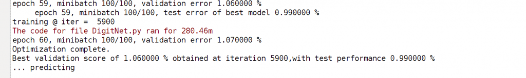
把预测结果提交给Kaggle之后,Score攀升至99.6%。由此可以看出,卷积神经网络相比随机森林而言还是强太多啊(好吧,另外一个因素是对于随机森林我根本没有做特征提取的工作)。此外,如果我的渣机强大一点的话,我们就能做更多次迭代,由此得到的准确率也可能更高吧。

如果大家对于手写数字识别这个TASK有更好的模型或者有一些其他的想法,欢迎交流昂!

参考文献

• 卷积神经网络（CNN）
• 卷积神经网络基本概念可参考Deep Learning（深度学习）学习笔记整理系列之（七）
• Convolutional Neural Networks (LeNet)